Complete Workflow Guide

This guide walks you through every step of the RRational workflow — from opening the app to exporting publication-ready HRV results.

---

Recommended: Scientific Workflow (Quigley 2024)

This workflow follows professor-reviewed best practices:

1. Import → Load data and verify participant detection
2. Inspect → Visual tachogram review for each participant
3. Segment → Time-based segmentation (5 min windows)
4. Detect → Run artifact detection on all validated sections
5. Assess → Per-segment quality grading — exclude segments with >10% artifacts
6. Analyze → HRV metrics on clean, assessed segments
7. Report → Always include: beat count, artifact rate, quality grade

---

Step 1: Launch & Create a Project

1.1 Start RRational

uv run streamlit run src/rrational/gui/app.py

The app opens at http://localhost:8501. You'll see the Data tab as the landing page.

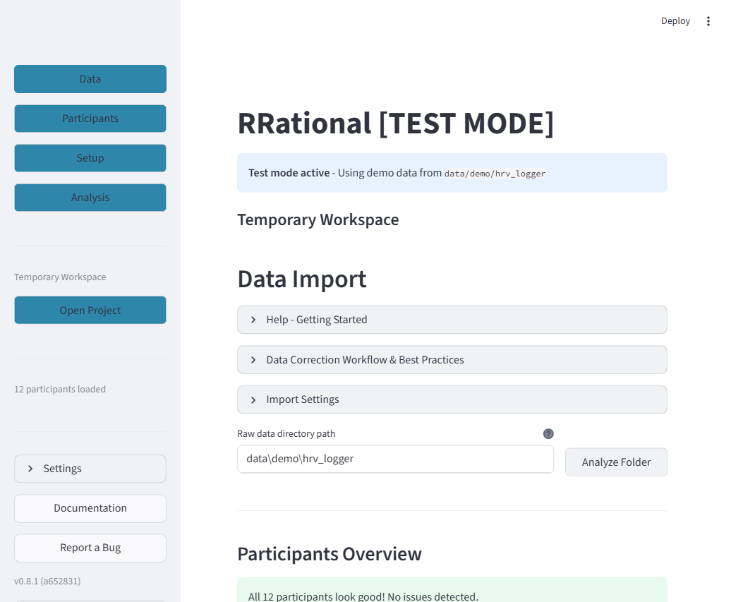
What you see: The Data Import page with three expandable help sections at the top ("Help - Getting Started", "Data Correction Workflow & Best Practices", "Import Settings"). Below is the Raw data directory path input field and the "Analyze Folder" button. In the sidebar (left): navigation buttons, project info, and at the bottom: Settings, Documentation, and Report a Bug.

Sidebar buttons explained:

Button	What it does
Data / Participants / Setup / Analysis	Switch between the four main tabs
Open Project (or Switch Project)	Open or switch to a different project
Settings	Expand to change plot resolution, colors, and data folder
Documentation	Opens the RRational documentation website
Report a Bug	Opens GitHub Issues to file a bug report

Data tab buttons explained:

Button / Element	What it does
Analyze Folder	Scans the raw data directory and loads all participant recordings
Help - Getting Started	Expandable section with usage instructions
Data Correction Workflow	Expandable section explaining the recommended correction pipeline
Import Settings	Expandable section to configure ID patterns, file formats, and import options

1.2 Create a Project

On the Welcome Screen (or via "Open Project" in the sidebar):

1. Click "Create New Project"
2. Click "Browse" → choose a folder (e.g., Documents/HRV_Studies/)
3. Enter a project name (e.g., MyStudy)
4. Select data sources: HRV Logger, VNS Analyse, or both
5. Click "Create Project"

Copy your data first

Copy your HRV recording files into the data/raw/hrv_logger/ or data/raw/vns/ subfolder before clicking "Analyze Folder".

---

Step 2: Import Data (Data Tab)

2.1 Load Recordings

1. Verify the Raw data directory path points to your data/raw/ folder
2. Click "Analyze Folder"
3. Wait for the scan to complete

2.2 Participants Overview

After loading, scroll down to the Participants Overview:

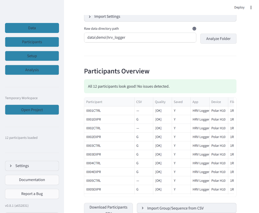
What you see: A green success bar ("All 12 participants look good!") followed by the participant table. Each row shows one participant with columns for: Participant (ID), CSV (import status), Quality ([OK] or warnings), Saved (Y/N), App (HRV Logger or VNS Analyse), Device (e.g., Polar H10), Files (number of RR/Events files), Date/Time (recording timestamp), Group (editable), Total Beats, Retained, Duplicates, Artifacts (%), and Duration (min).

Table columns explained:

Column	Meaning
Participant	Auto-extracted ID from filename (e.g., 0001CTRL)
Quality	[OK] = no issues, warnings indicate problems
Saved	Y = events have been saved to disk
Total Beats	Total number of RR intervals in the recording
Retained	Beats remaining after duplicate removal
Group	Study group — editable directly in the table

2.3 Below the Table

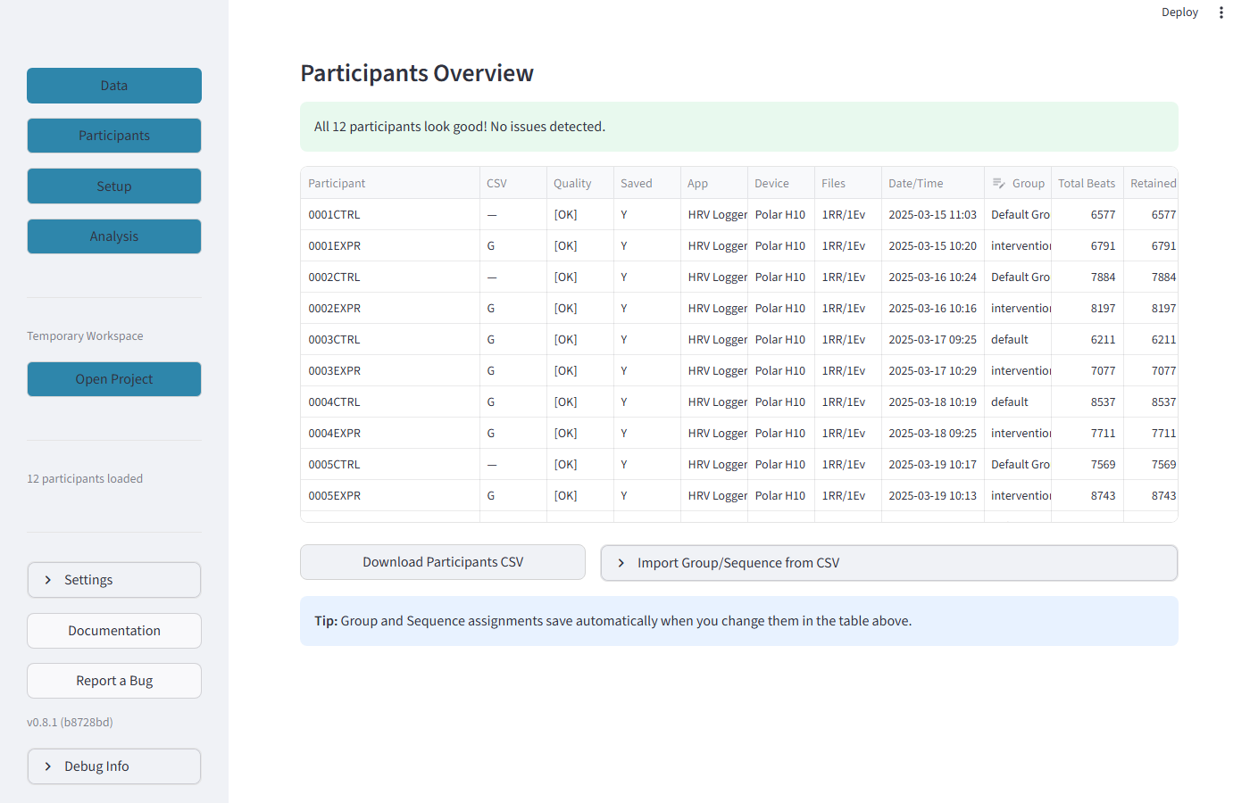
Below the table you'll find two buttons and a tip:

Button	What it does
Download Participants CSV	Downloads the participant table as a CSV file for external use
Import Group/Sequence from CSV	Opens an expandable section to bulk-import group and sequence assignments from a study master CSV

---

Step 3: Review Participants (Participants Tab)

Click "Participants" in the sidebar.

3.1 Participant Header

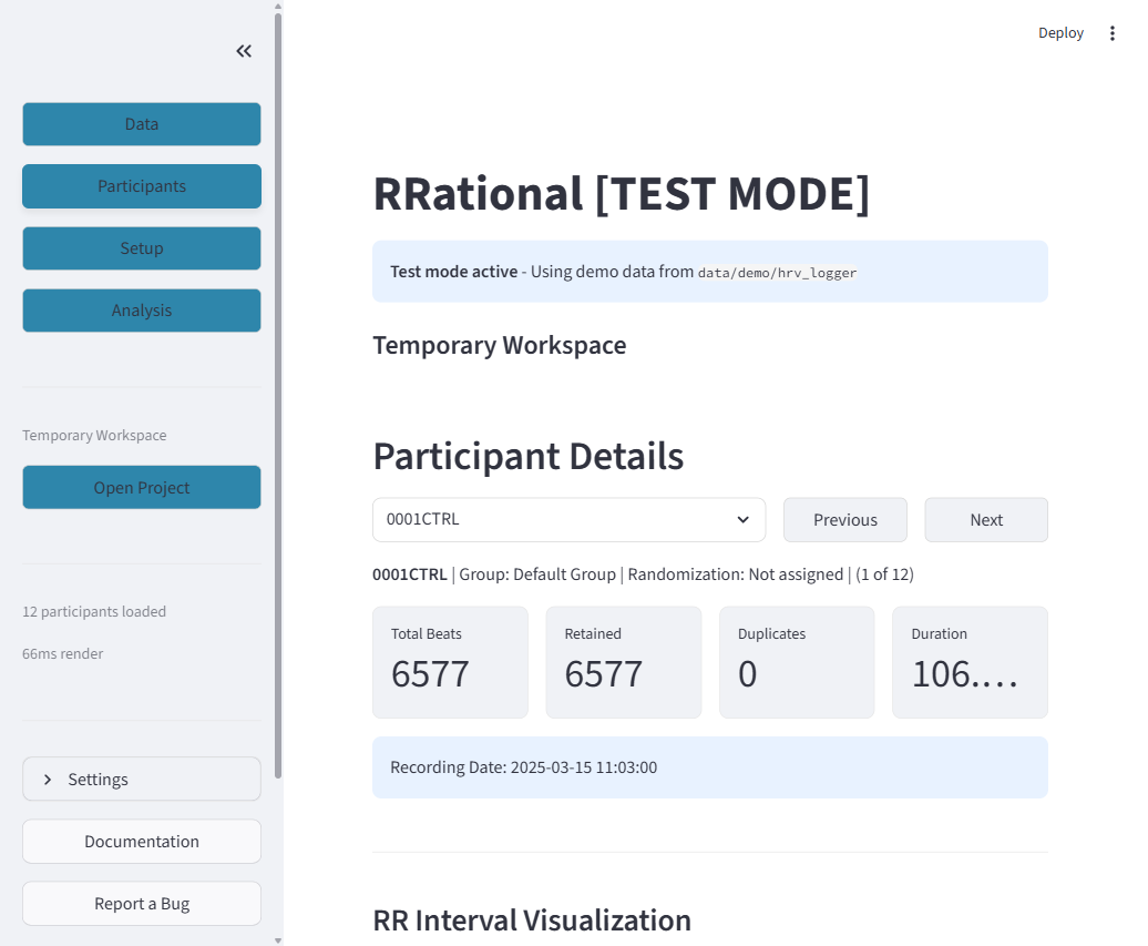
What you see: A dropdown to select a participant (e.g., "0001CTRL"), Previous and Next buttons for navigation, a summary line ("Group: Default Group | Randomization: Not assigned | 1 of 12"), and four metric cards.

Metric cards explained:

Card	Meaning
Total Beats	Total RR intervals in the recording
Retained	Beats kept after duplicate removal
Duplicates	Number of duplicate timestamps removed
Duration	Total recording duration in minutes

3.2 Mode Selector & Plot Options

Below the metrics, you'll see the interaction modes and plot settings:

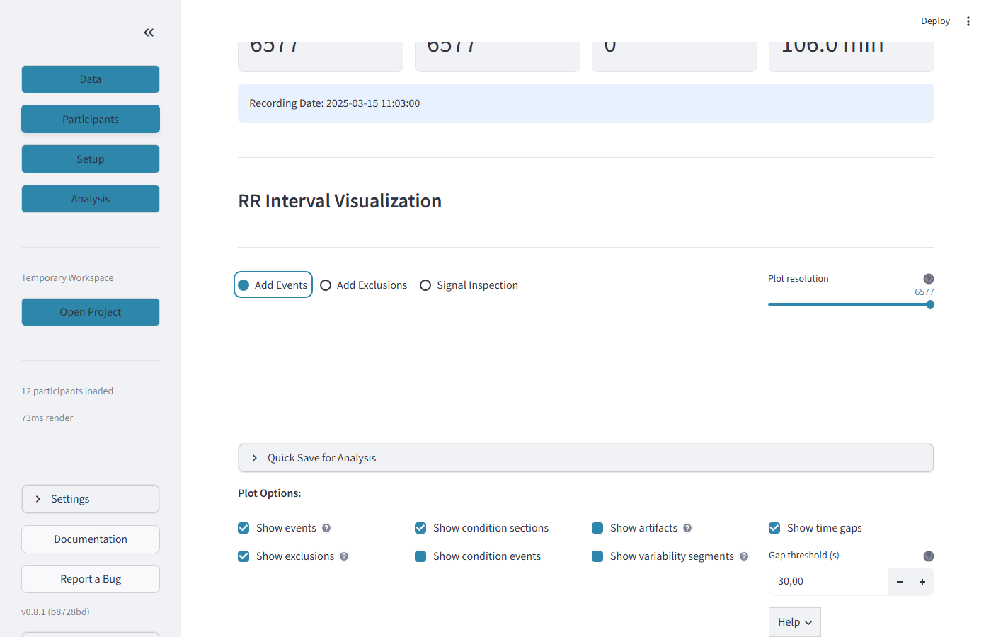
What you see: The RR Interval Visualization heading, three mode buttons ("Add Events", "Add Exclusions", "Signal Inspection"), a plot resolution selector, and the "Quick Save for Analysis" expander. Below are the Plot Options checkboxes.

Mode buttons explained:

Mode	What it does
Add Events	Click anywhere on the tachogram to add a new event marker at that timestamp
Add Exclusions	Click two points on the tachogram to mark a time range for exclusion from analysis
Signal Inspection	Enables detailed artifact inspection with zoom and pan capabilities

Plot Options checkboxes:

Checkbox	What it shows/hides
Show events	Vertical dashed lines at event timestamps (measurement start, pause, etc.)
Show condition sections	Colored background regions for repeating experimental conditions
Show artifacts	Orange markers for detected artifacts — also reveals the Detect New Artifacts expander
Show time gaps	Gray shading for recording interruptions (HRV Logger only)
Show exclusions	Red shading for manually excluded time ranges
Show condition events	Individual start/end event markers for conditions
Show variability segments	Color-coded regions indicating local variability (green=stable, orange=moderate, red=high)

Other controls:

Control	What it does
Gap threshold (s)	Minimum gap duration (in seconds) to display. Default: 15s
Help	Dropdown with explanation of keyboard shortcuts and interaction modes
Refresh	Reloads the current participant's data and redraws the plot
Quick Save for Analysis	Expander to save artifact markings without full export

3.3 The Tachogram

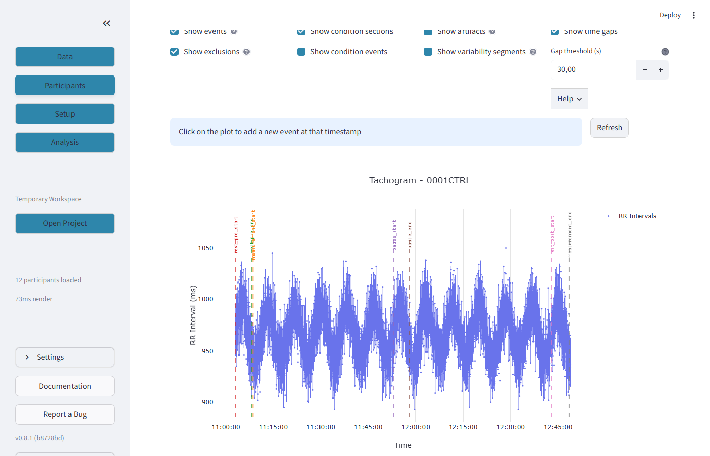
What you see: The tachogram plot with RR intervals (ms) on the Y-axis and time on the X-axis. The blue line traces the heart rhythm. Vertical dashed lines mark events. Orange dots are detected artifacts. The plot title shows "Tachogram - 0001CTRL" and the legend identifies "RR Intervals".

What to look for:

• Regular oscillations in the blue line = normal respiratory sinus arrhythmia
• Flat lines or sudden jumps = potential artifacts or movement
• Orange dots = detected ectopic, missed, or extra beats
• Dashed vertical lines = event markers (measurement start, pause, etc.)

---

Step 4: Artifact Detection

Why artifacts matter

Even a small number of artifacts can dramatically distort HRV metrics. Always detect and assess artifacts before analysis.

4.1 Enable Artifacts

1. Check the "Show artifacts" checkbox in Plot Options
2. This reveals the "Detect New Artifacts" expander below the plot

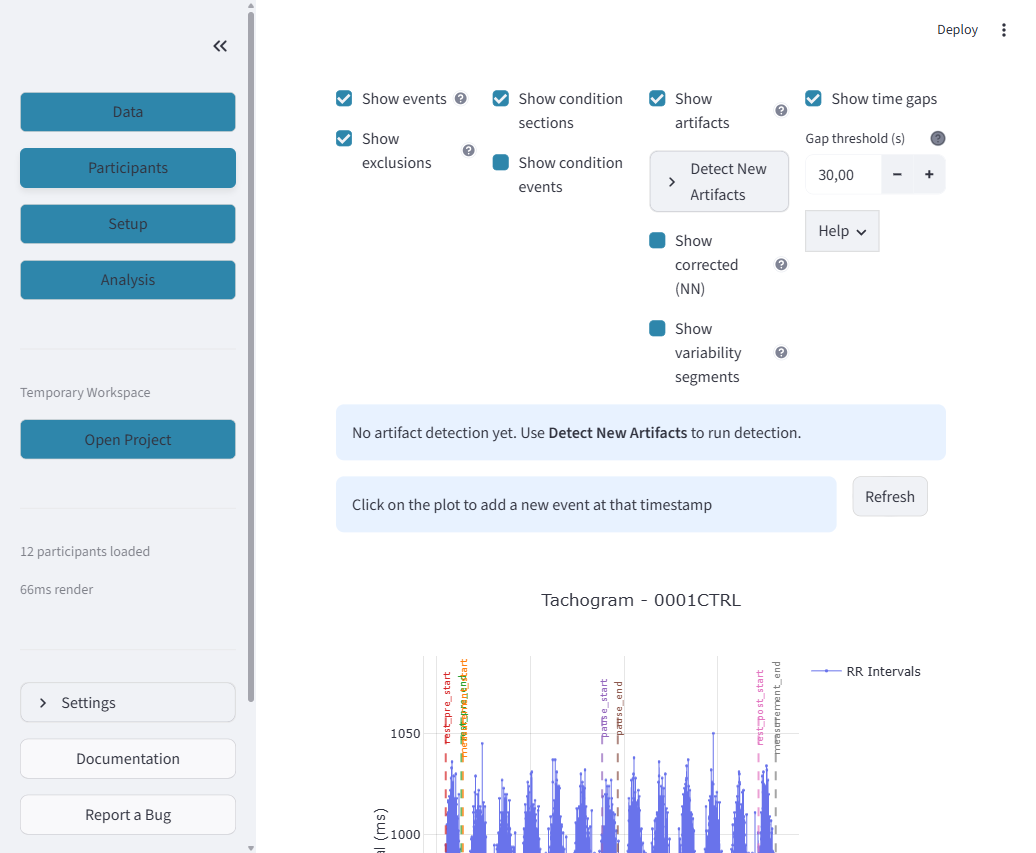
After enabling "Show artifacts", orange markers appear on the tachogram showing where the algorithm detected problematic beats.

4.2 Artifact Detection Settings

Expand "Detect New Artifacts" to configure detection:

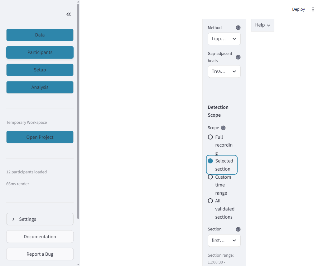
What you see: The detection panel with Method, Gap handling, Detection Scope, Section selector, and Segment Sizing options.

Settings explained:

Setting	Options	Recommended
Method	Lipponen 2019 (segmented)	Lipponen 2019 — current gold standard
Gap-adjacent beats	Treat as segment boundaries / Include in detection	Treat as segment boundaries — prevents false positives near gaps
Detection Scope	Full recording / Selected section / Custom time range / All validated sections	All validated sections — ensures same segments for detection and analysis
Segment Sizing	Adaptive / Preset / Manual	Adaptive — automatically calculates optimal window size

4.3 Detection Scope

The Detection Scope is critical for the scientific workflow:

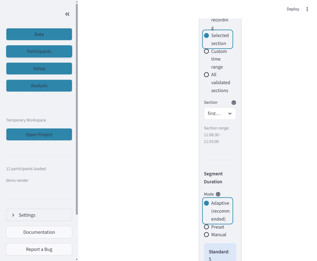
What you see: Four radio buttons for scope selection, a section dropdown (when "Selected section" is chosen), and the time range display.

Scope	What it does	When to use
Full recording	Detects across the entire recording	Quick overview, exploratory analysis
Selected section	Detects within one specific section	When you only need one section
Custom time range	Manual start/end time selection	For unusual recording structures
All validated sections	Detects separately for each validated section	Recommended — scientific workflow

4.4 Run Detection

Click "Run Detection" and review the results.

4.5 Section Validation & Data Integrity

Scroll down to see the Section Validation results:

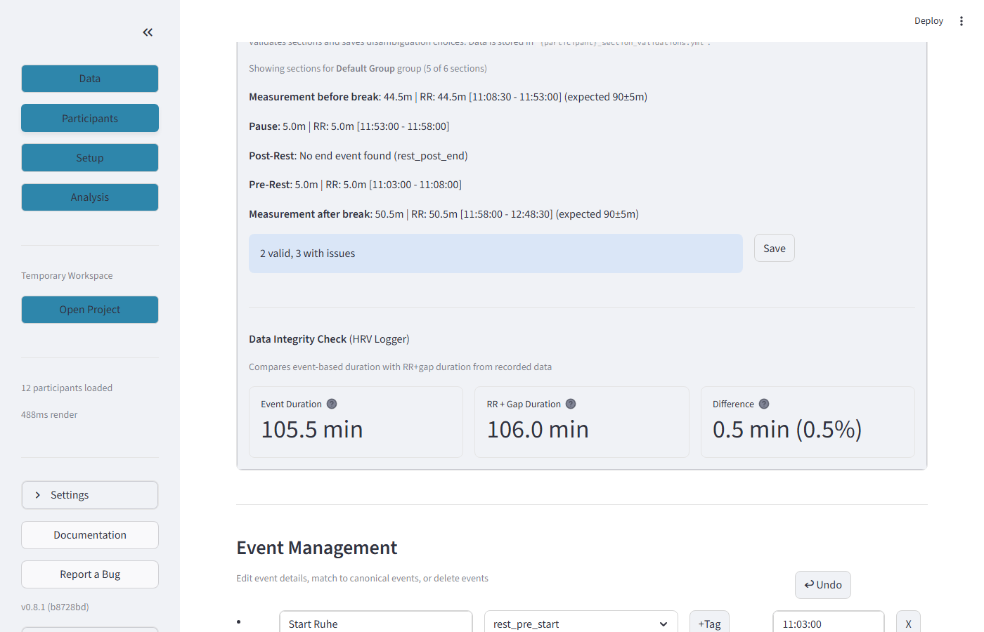
What you see: Each defined section with its validation status. For this participant: "Measurement before break" (44.5 min), "Pause" (5.0 min), "Post-Rest" (no end event found), "Pre-Rest" (5.0 min), "Measurement after break" (50.0 min). The summary shows "2 valid, 3 with issues" and a Save button.

Section validation indicators:

Indicator	Meaning
Bold section name + duration	Section is valid, events found
"No end event found"	End event is missing — section cannot be analyzed
"expected X±Ym"	Shows expected duration with tolerance
2 valid, 3 with issues	Summary of validation results

Below the section list, the Data Integrity Check compares: Event Duration (from event timestamps: 105.5 min) vs RR+Gap Duration (from summing all RR intervals and gaps: 106.0 min). The Difference (0.5 min, 0.5%) should be small — large differences indicate data corruption.

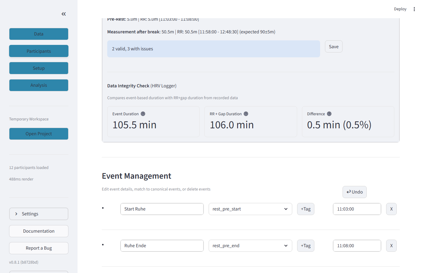
4.6 Event Management

What you see: The Event Management section where you can edit, reorder, or delete events. Each event row shows: a drag handle (bullet), the raw label (e.g., "Start Ruhe"), the canonical name dropdown (e.g., "rest_pre_start"), a +Tag button, and the timestamp (e.g., "11:03:00"). The X button deletes an event.

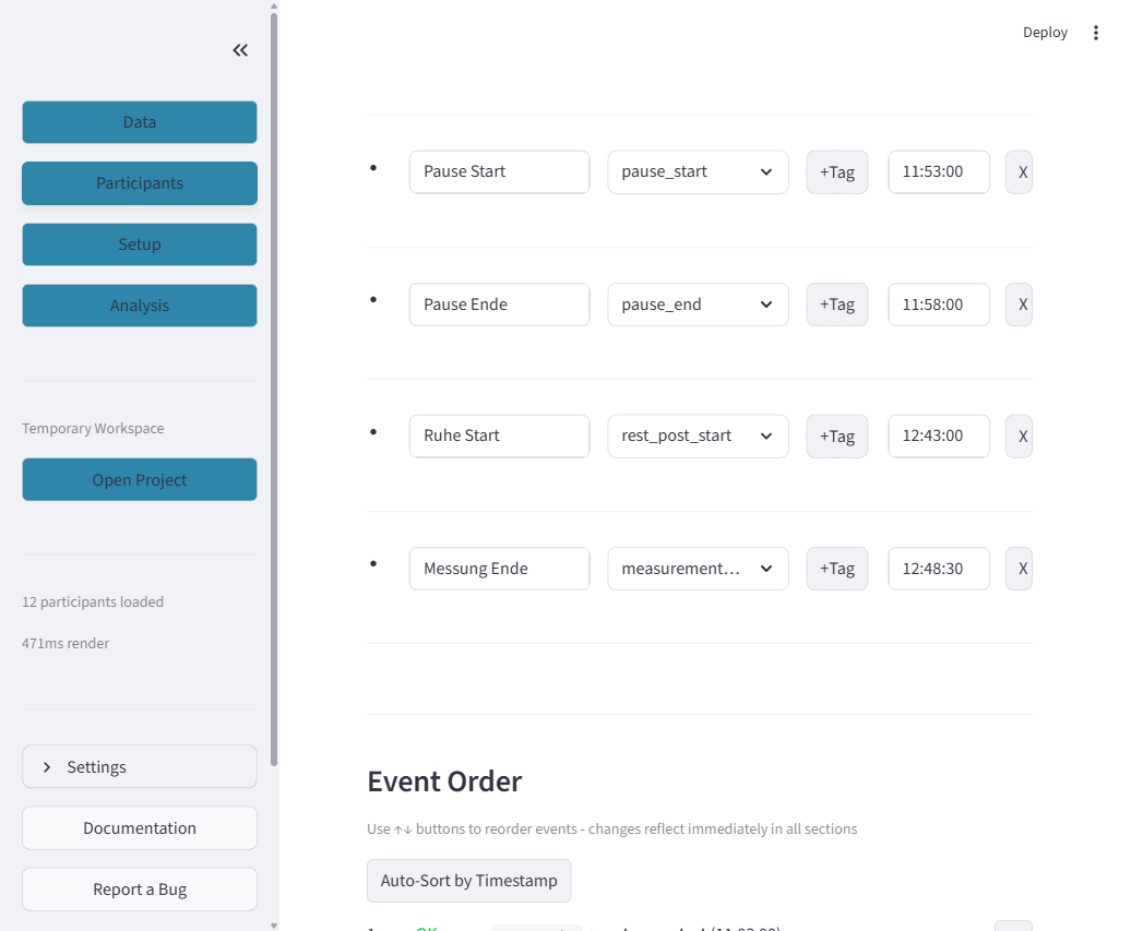
4.7 Event List Detail

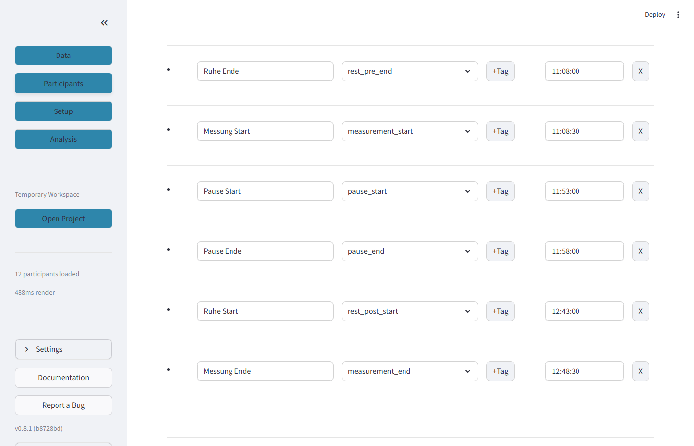
Each event in the list has:

Element	What it does
Raw label (left text field)	The original event name from the recording file (e.g., "Ruhe Ende")
Canonical name (dropdown)	The standardized event name (e.g., "rest_pre_end") — used for section matching
+Tag button	Add a tag/label to this event
Timestamp (right field)	The event time (HH:MM:SS)
X button	Delete this event

4.8 Event Mapping Status

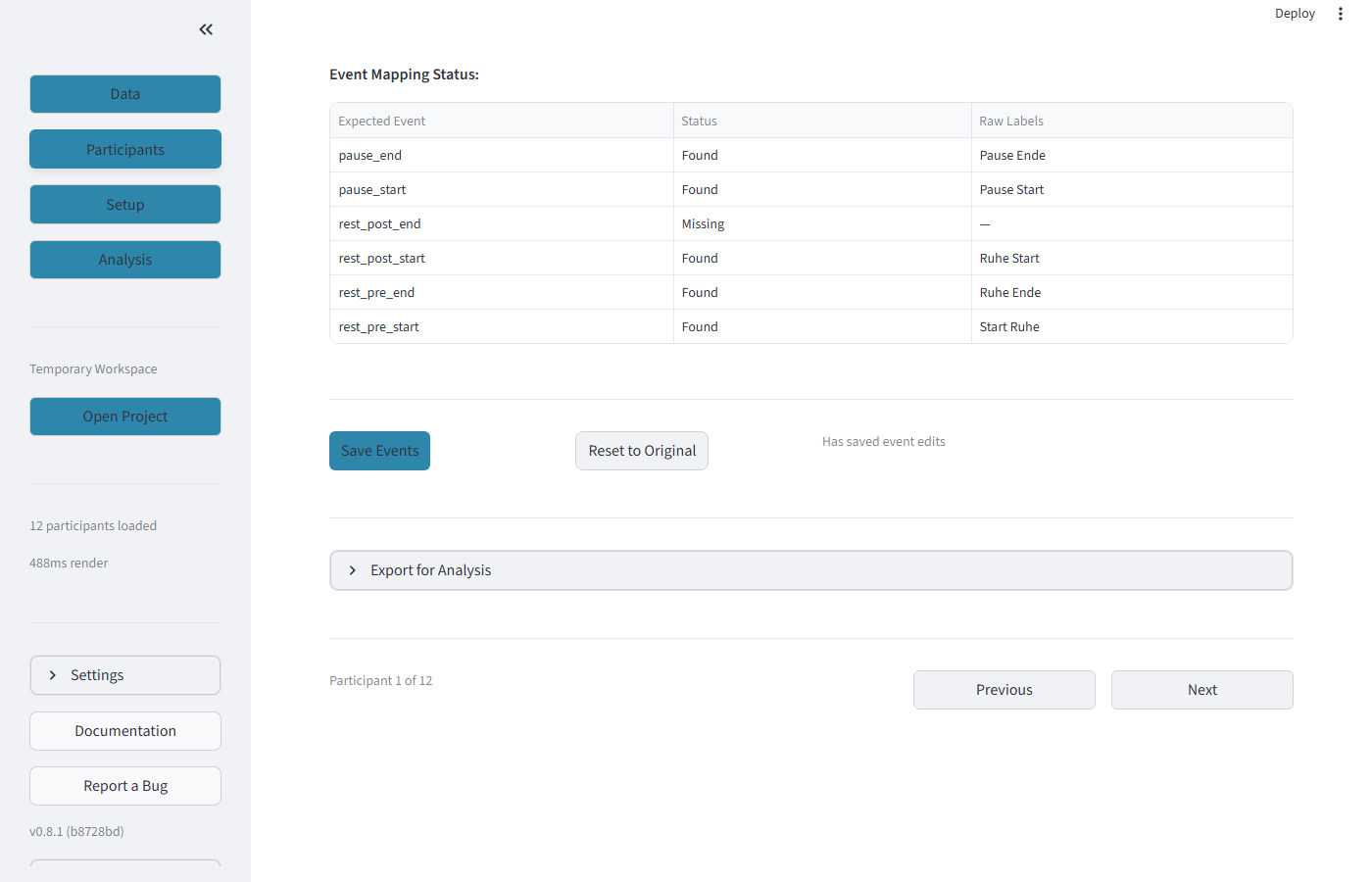
The Event Mapping Status table shows which expected events were detected. "Found" (green) means the event was matched. "Missing" (red) means no matching event exists — you may need to add it manually or update synonyms in Setup > Events.

Button	What it does
Save Events	Persist all event changes to disk
Reset to Original	Undo all manual changes and restore original events

4.9 Export for Analysis

The Export for Analysis section saves a .rrational file containing corrected RR intervals, artifact indices, quality metrics, and a full audit trail. This file can be reloaded in the Analysis tab.

Quality Grading (Quigley 2024)

Grade	Artifact Rate	Action
Excellent	<2%	Include as-is
Good	2-5%	Include, apply correction
Fair	5-10%	Include with caution
Poor	>10%	Exclude from analysis

---

Step 5: Configure Study (Setup Tab)

Click "Setup" in the sidebar. Four sub-tabs are available via radio buttons: Events, Groups, Sequences, Sections.

5.1 Events

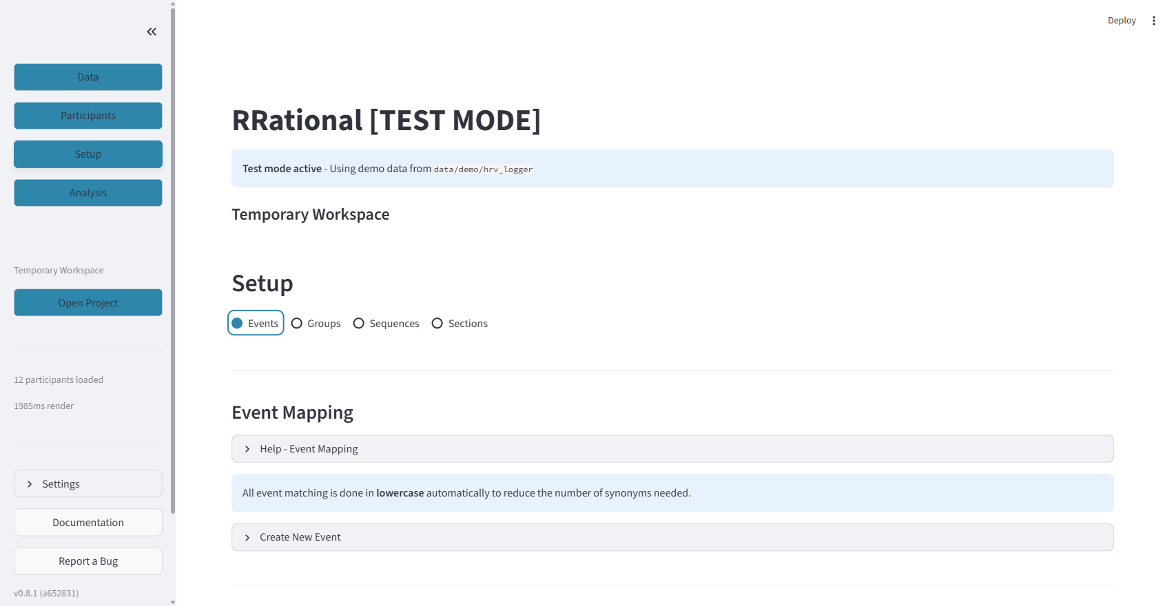
What you see: The Events sub-tab (selected in the radio buttons). The "Event Mapping" section with a help expander, an info bar about case-insensitive matching, and a "Create New Event" expander.

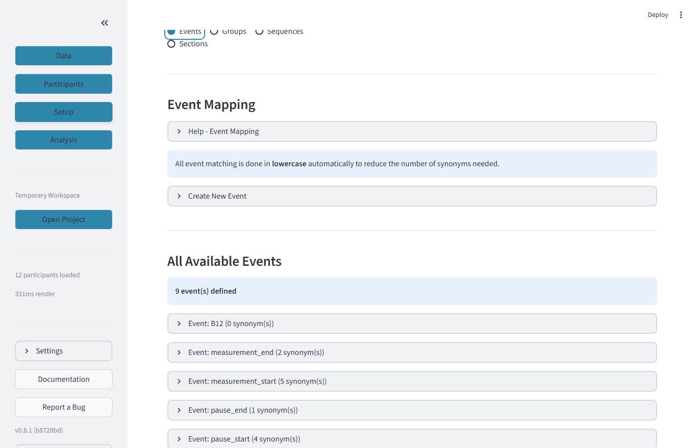
Scrolling down reveals the event definitions table. Each event has a canonical name (e.g., measurement_start), synonyms for fuzzy matching (comma-separated), and a regex pattern for advanced matching.

Button	What it does
Create New Event	Add a new canonical event name with synonyms
Save Event Changes	Persist all changes to the event configuration
Download Events CSV	Export event definitions as CSV

5.2 Groups

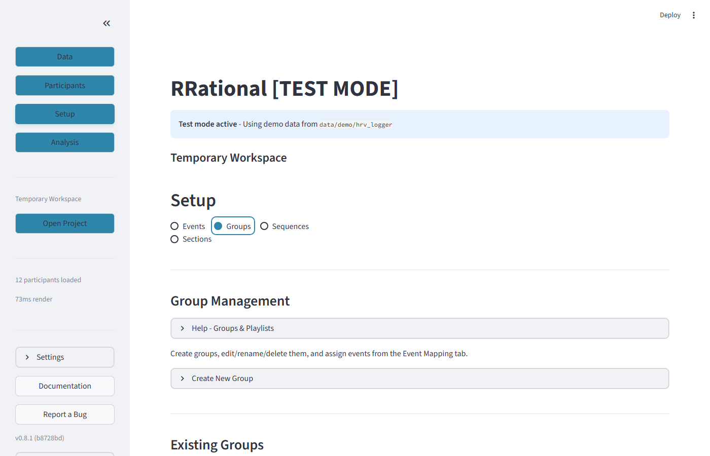
What you see: The Groups sub-tab showing "Group Management". A help expander explains groups. Below is "Create New Group" and a list of existing groups.

Button	What it does
Create New Group	Add a new study group (e.g., "control", "experimental")
Save Changes	Save group label and event assignments
Delete	Remove a group (does not delete participant data)

5.3 Event Sequences

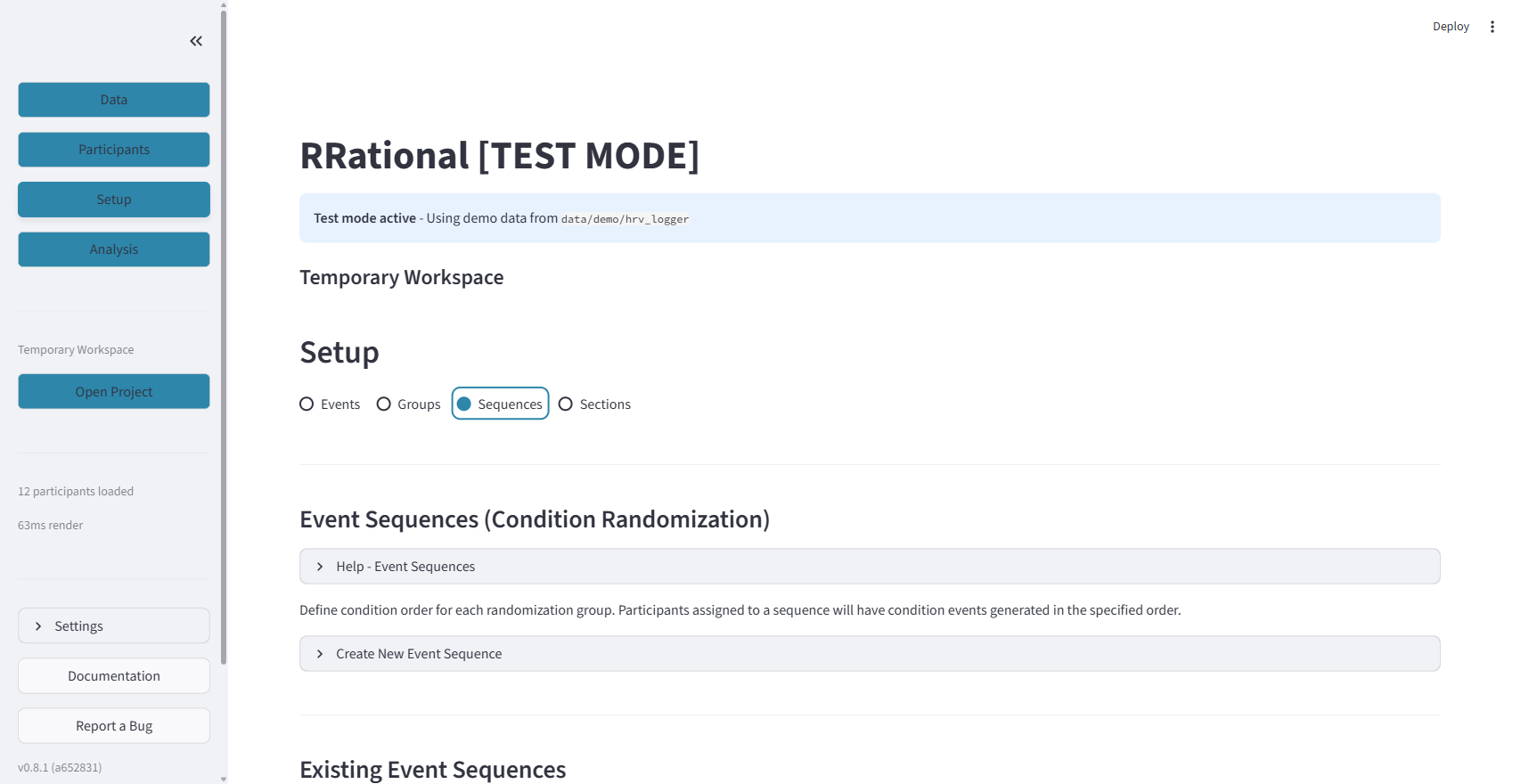
What you see: The Sequences sub-tab showing "Event Sequences (Condition Randomization)". This is where you define the order of repeating conditions for randomization studies.

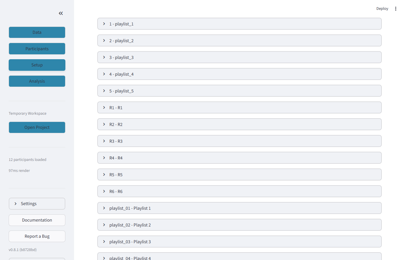
Each sequence shows its label, condition order as arrows (e.g., "music_1 → music_2 → music_4 → music_3"), and buttons to edit or delete. Participants assigned to this sequence are listed below.

Button	What it does
Create Event Sequence	Add a new sequence with condition order
Save Changes	Update label and condition order
Delete	Remove the sequence and unassign participants

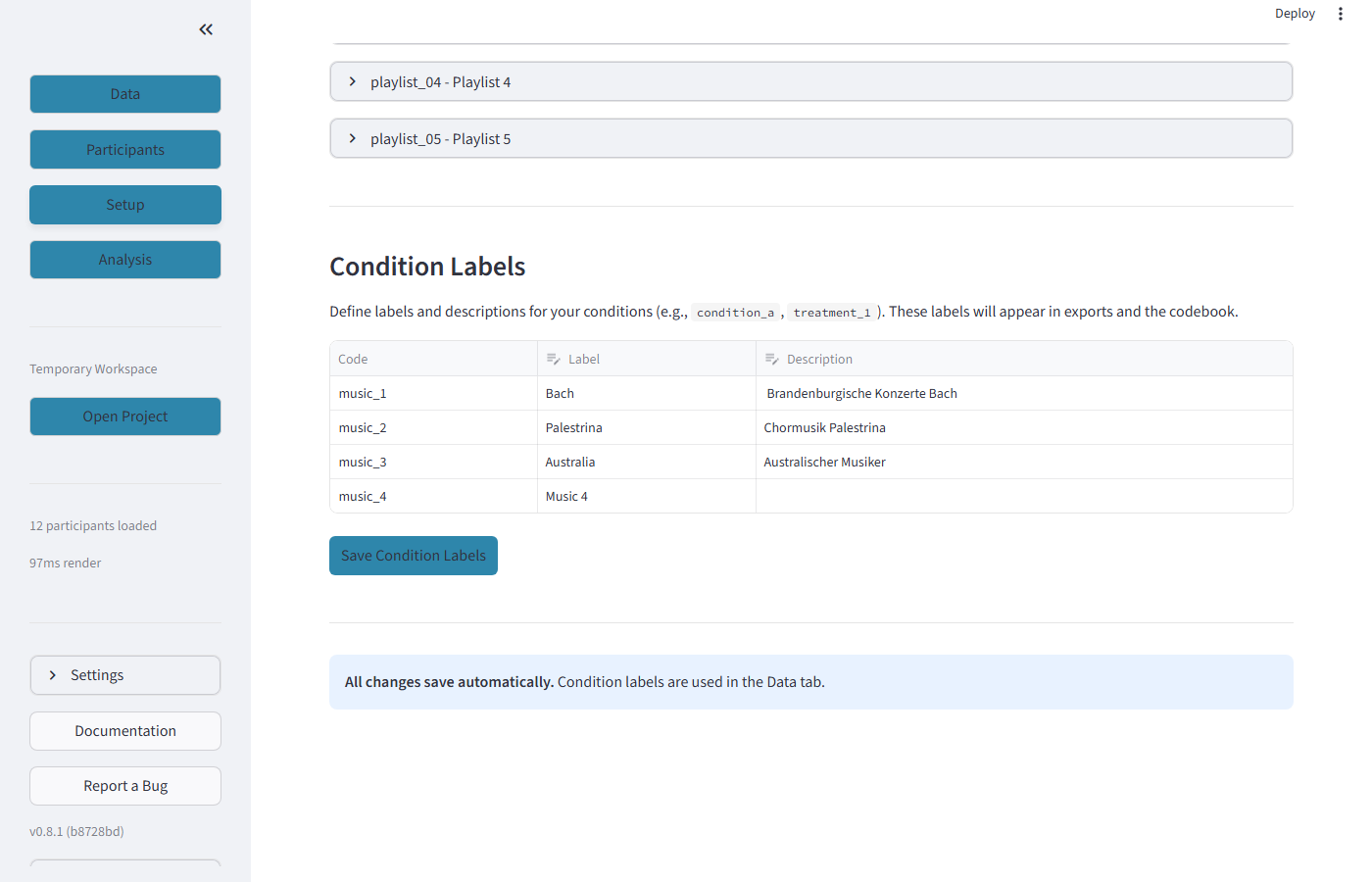
Below the sequences, the Condition Labels table lets you define display names. For example, internal code "music_1" can be labeled "Bach" with description "Brandenburgische Konzerte Bach".

Button	What it does
Save Condition Labels	Persist label and description changes

5.4 Sections

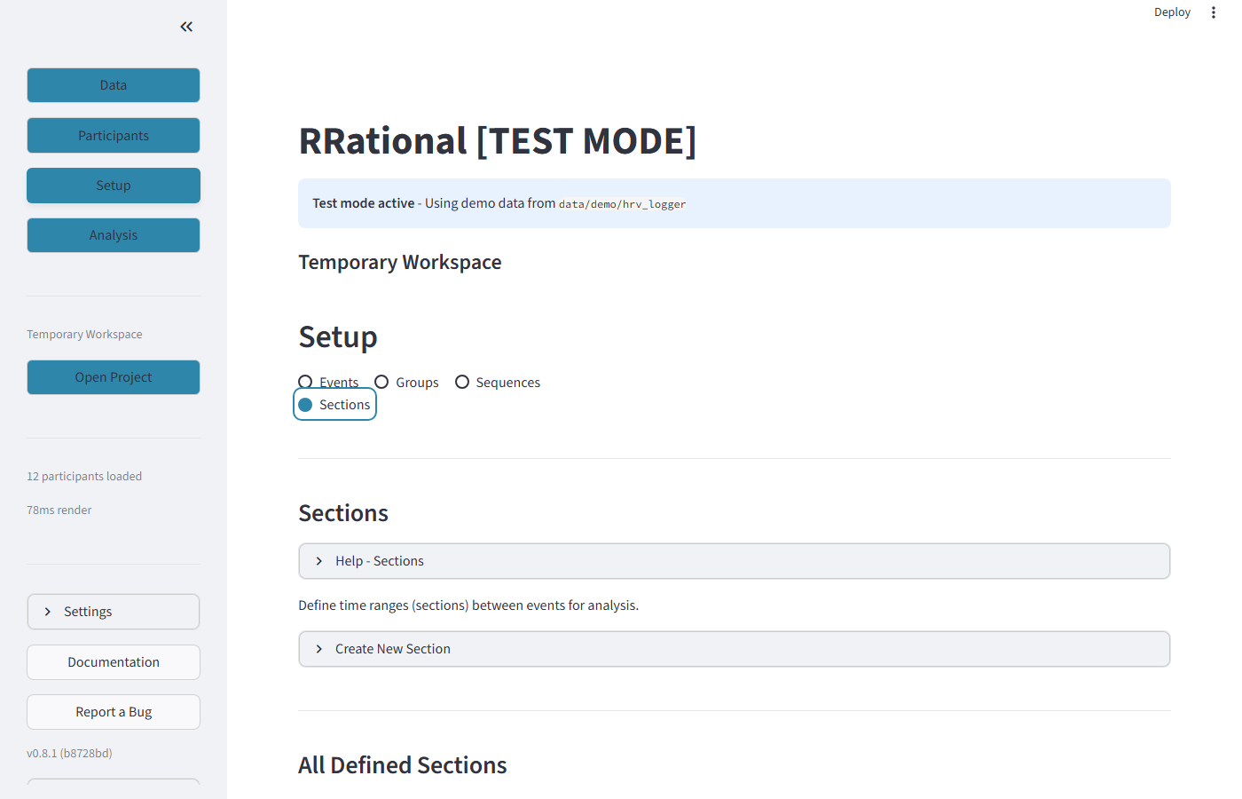
What you see: The Sections sub-tab where you define analysis time windows. Each section has a Code, Label, Start/End Event(s), expected Duration, and Tolerance.

Field	What it means
Code	Internal identifier (e.g., baseline)
Label	Display name (e.g., "Baseline Rest")
Start Event(s)	Comma-separated event names that start this section
End Event(s)	Comma-separated event names that end this section (first match wins)
Duration (min)	Expected duration for validation
Tolerance (min)	How much the actual duration may deviate

---

Step 6: Analyze HRV (Analysis Tab)

Click "Analysis" in the sidebar.

6.1 Choose Analysis Mode

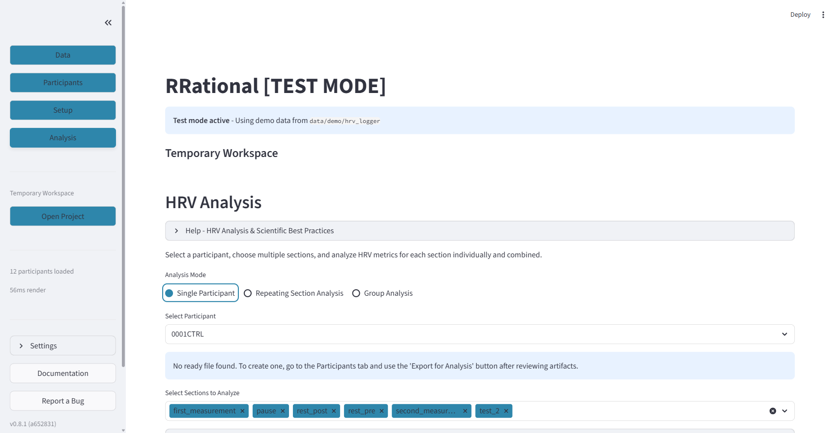
What you see: Four radio buttons for analysis mode, a participant selector, and a section multiselect. The available sections are pre-selected based on validation.

Frequency-domain pipeline selector

Above the mode selector, a single global Frequency-domain pipeline dropdown (NeuroKit2 default vs Kubios-compatible) applies to all four analysis modes. See the Kubios Compatibility Guide.

Mode	What it does	When to use
Single Participant	Analyze one participant's sections individually	Detailed per-participant analysis
Repeating Section Analysis	Protocol-based repeating condition comparison	Studies with repeating conditions (e.g., music, stimuli)
Group Analysis	Batch comparison across study groups	Group-level statistical comparisons
Sequence Comparison	Compare HRV across event sequences and conditions	Counterbalanced designs, condition-order effects

6.2 Single Participant Settings

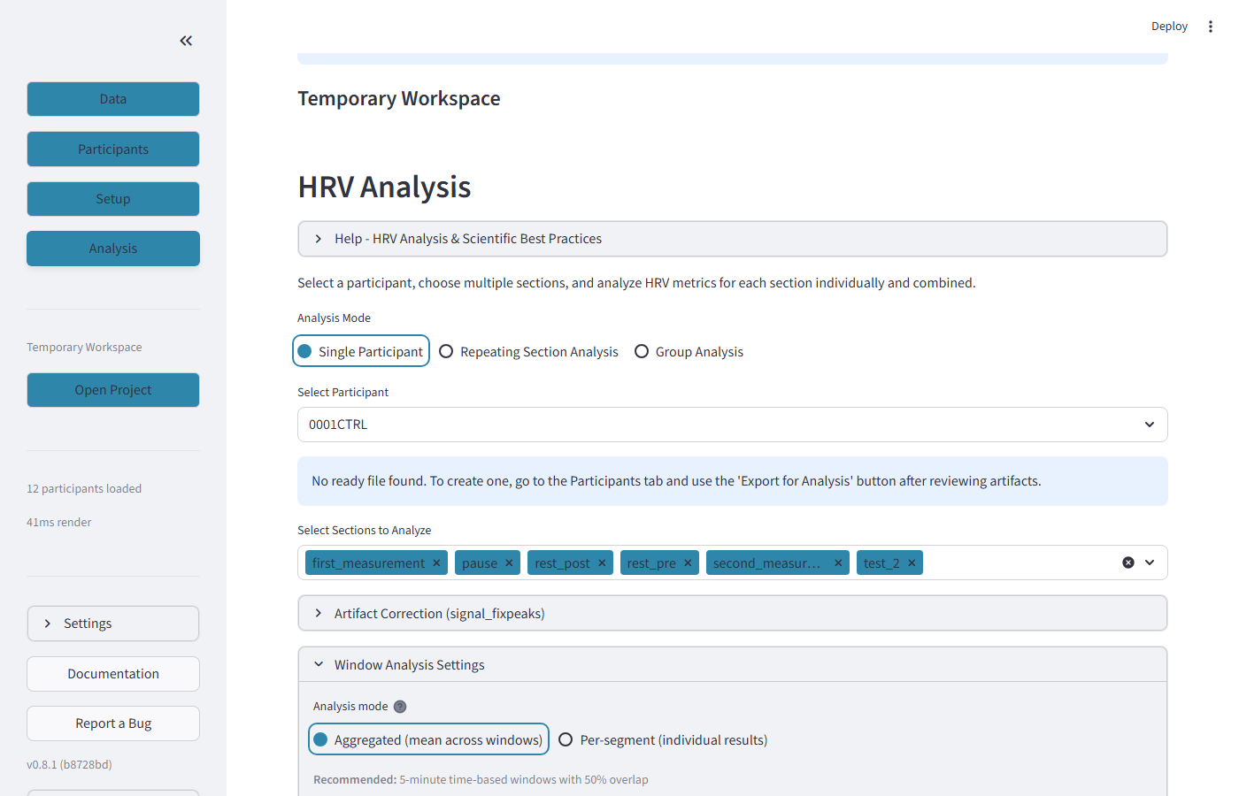
What you see: Participant dropdown, section multiselect (all validated sections pre-selected), artifact correction expander, and analysis mode options (Aggregated vs Per-segment).

Setting	What it does
Select Participant	Choose which participant to analyze
Select Sections to Analyze	Choose which sections to include (defaults to all validated)
Artifact Correction	Enable NeuroKit2 Kubios algorithm for artifact correction
Aggregated	One result per section (combines all windows)
Per-segment	Separate results for each time-based segment within a section
Analyze HRV	Run the analysis and show results

6.3 Repeating Section Analysis

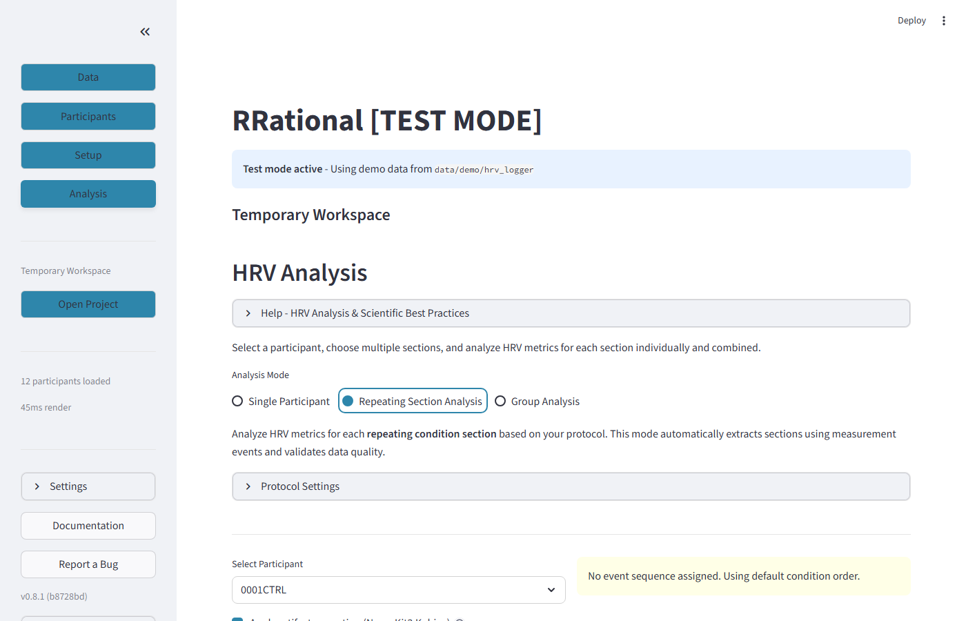
What you see: The "Repeating Section Analysis" mode with Protocol Settings expander and participant/sequence selection. A warning appears if no event sequence is assigned.

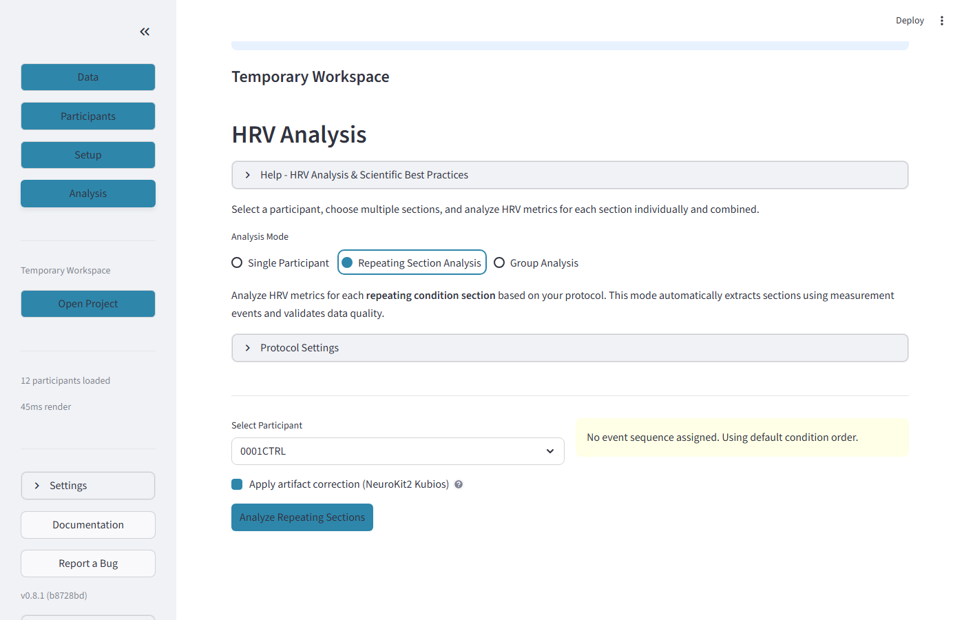
The Protocol Settings define the expected recording structure: total duration, section length, number of pre/post-pause sections, minimum valid duration and beats, and how to handle duration mismatches.

6.4 Group Analysis

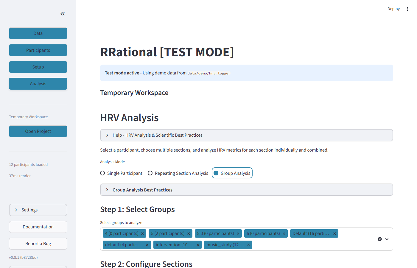
What you see: Group Analysis mode where you select two or more study groups, choose a metric preset, and run a batch comparison across all participants in those groups.

Group Analysis reads each participant's .rrational file once and aggregates the per-section metrics across the group. Results appear in three tabs:

Data tab — a descriptive table of per-group means and dispersion for every selected metric, with CSV export.

Statistics tab — descriptive statistics plus a Hypothesis Tests panel. The appropriate test is selected automatically based on the number of groups and a normality check (Shapiro-Wilk):

Groups	Distribution	Test	Effect size
2	normal	Welch's t-test	Cohen's d
2	non-normal	Mann-Whitney U	—
3+	normal	one-way ANOVA	η² (eta-squared)
3+	non-normal	Kruskal-Wallis	η²

When several metrics are tested together, p-values are adjusted for multiple comparisons (Holm by default; Bonferroni and Benjamini-Hochberg FDR are also available). Frequency-domain metrics (LF, HF, VLF, Total Power) are log-transformed before parametric testing because their distributions are log-normal.

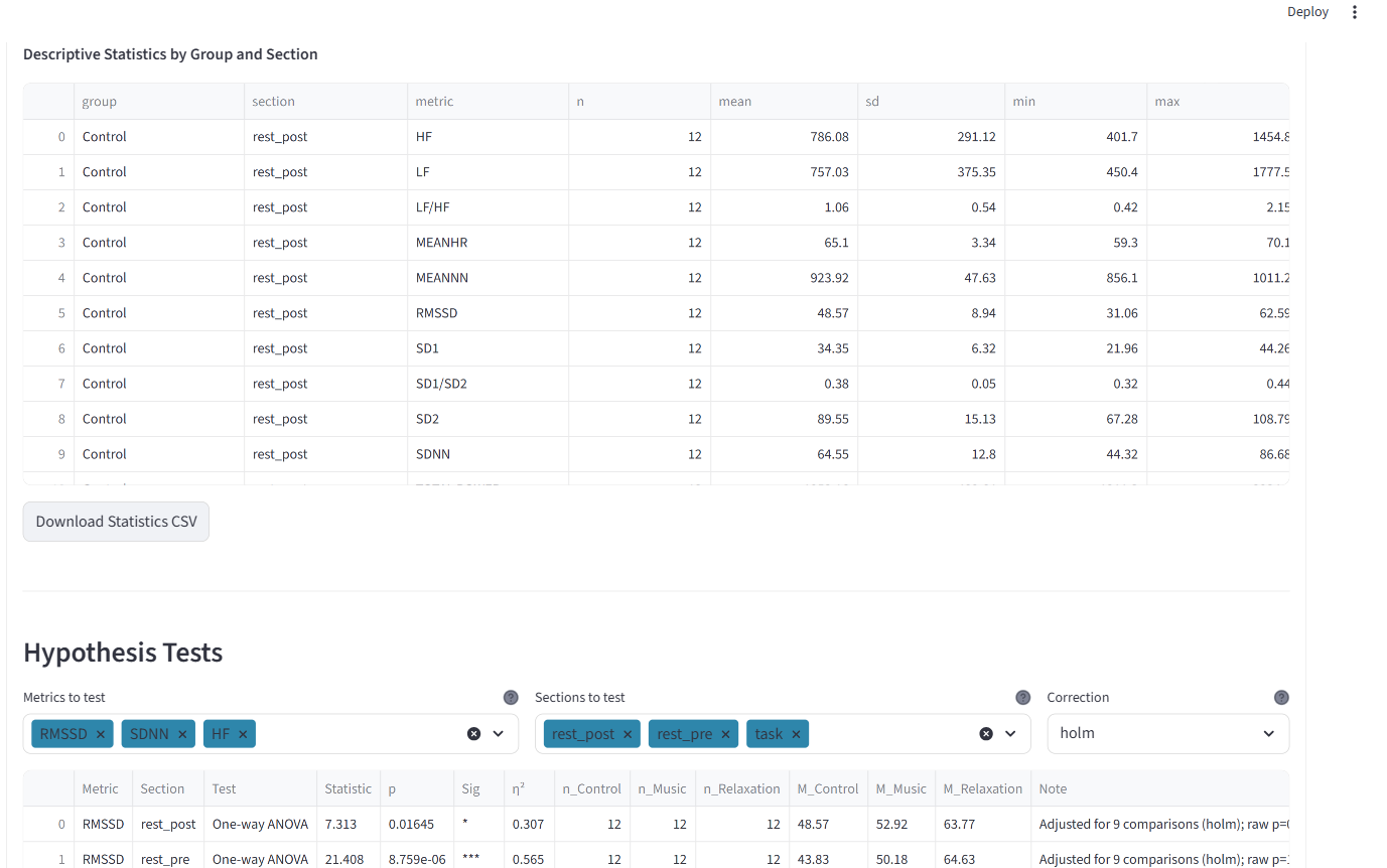
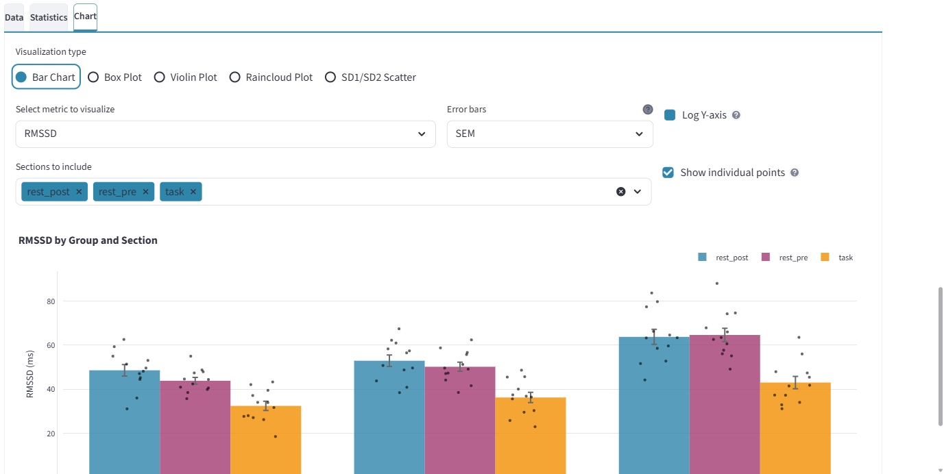
Chart tab — bar charts, box plots, violin plots, raincloud plots and SD1/SD2 scatter, with options to:

• choose the error-bar type (SEM default, SD, CI95, or None),
• overlay individual data points behind the summary statistics,
• use a log Y-axis (enabled automatically for log-normal metrics such as LF/HF).

Cached results. A completed analysis can be saved to the project (data/processed/group_analysis_results.yml). When a cache exists, a "Cached results available" banner offers Load (instant) or Delete, with the last-saved timestamp; the analysis can also be exported as an HTML report. Because each .rrational file is read only once per participant, a fresh run is substantially faster than per-metric loading.

6.5 Sequence Comparison

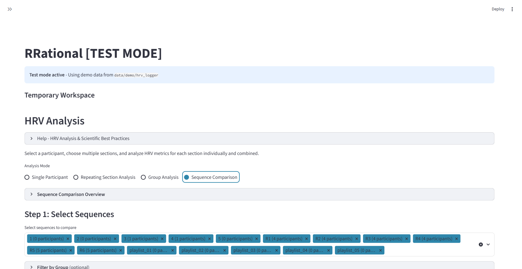
What you see: The "Sequence Comparison" mode with all event sequences listed, showing participant counts per sequence. An optional "Filter by Group" expander allows cross-group comparisons.

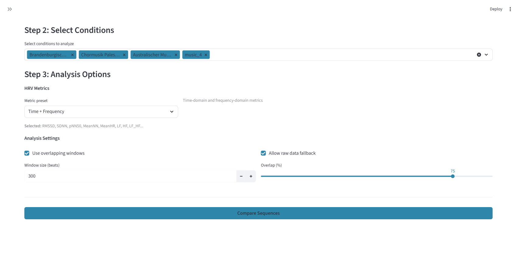
Step 2 shows conditions to compare (extracted from sequence definitions). Step 3 provides metric presets and analysis settings similar to Group Analysis.

Setting	What it does
Select Sequences	Choose which event sequences to compare
Filter by Group	Optionally add group dimension to comparisons
Select Conditions	Choose which experimental conditions to analyze
Compare Sequences	Run the comparison and display results with charts

Results are displayed in Data, Statistics, and Chart tabs, using the same chart types as Group Analysis (bar charts, box plots, violin plots, raincloud plots, SD1/SD2 scatter).

6.6 Power Spectrum (PSD)

In the Participants tab, below the tachogram, an expandable Power Spectrum (PSD) section shows the frequency-domain analysis for the current participant.

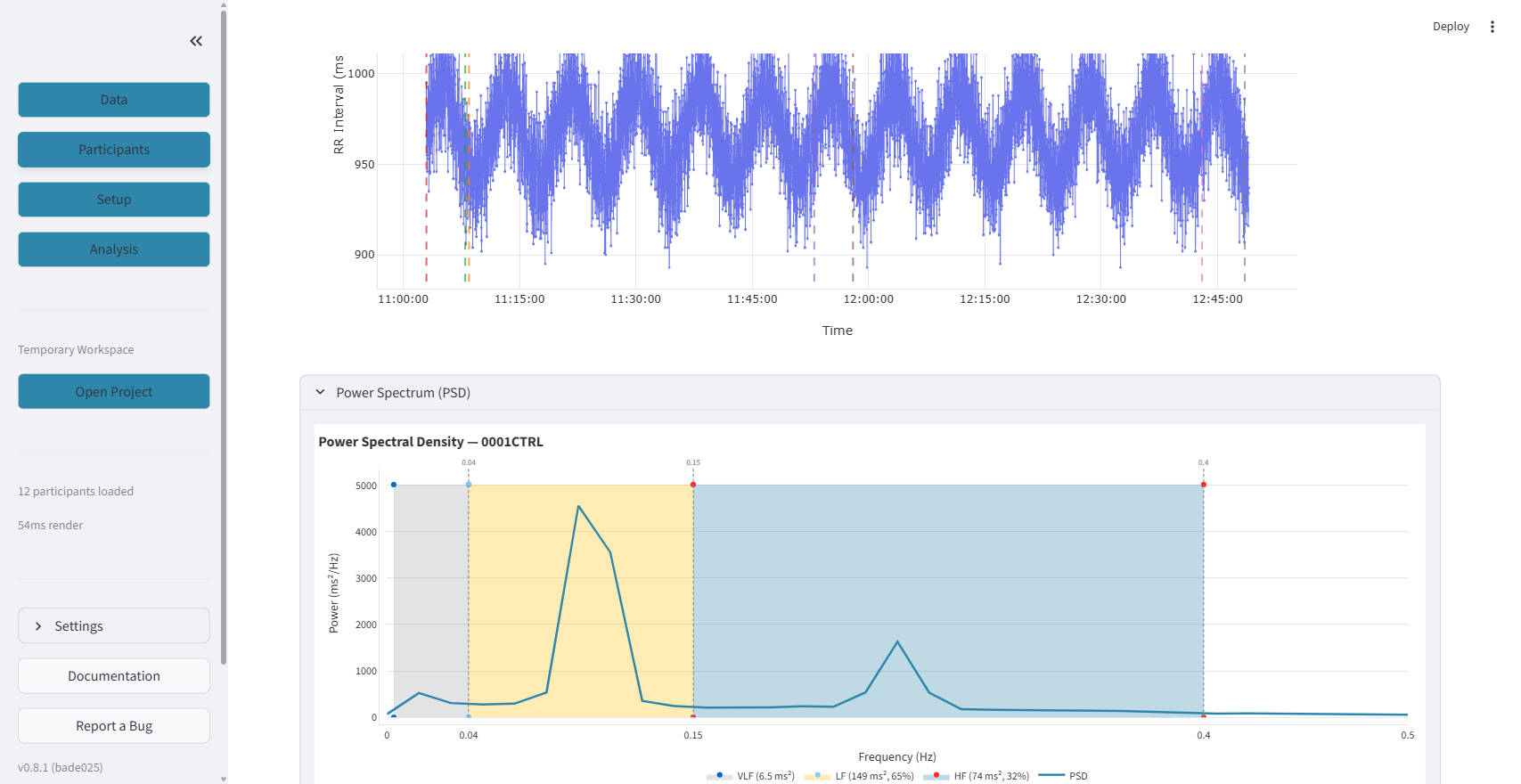
The Power Spectral Density plot shows VLF (gray), LF (yellow), and HF (blue) frequency bands with power values and percentages. The PSD line shows the Welch-estimated power distribution.

Band	Frequency Range	What it reflects
VLF	0.003–0.04 Hz	Thermoregulation, hormonal
LF	0.04–0.15 Hz	Both sympathetic and parasympathetic + baroreflex
HF	0.15–0.4 Hz	Parasympathetic (vagal) activity

Note

The PSD requires at least 100 beats (300+ recommended). It uses the full (non-downsampled) RR data for accurate frequency estimation.

6.7 Report Export

Analysis reports can be downloaded in two formats:

Format	What it includes
Markdown (.md)	Text-based report with tables — suitable for research documentation
HTML	Standalone file with professional styling, summary cards, and optionally embedded charts — suitable for sharing and printing

For Single Participant analysis, reports include data source, cleaning parameters, artifact correction details, section information, and all computed HRV metrics.

For Group Analysis, HTML reports include participant counts, descriptive statistics tables, and individual results — all in a single self-contained file.

6.8 HRV Metrics Reference

Metric	Domain	What It Tells You
RMSSD	Time	Beat-to-beat variability — primary parasympathetic marker
SDNN	Time	Overall HRV — reflects all sources of variability
pNN50	Time	Percentage of successive intervals differing >50 ms
Mean HR	Time	Average heart rate in beats per minute
LF	Frequency	Low-frequency power (0.04-0.15 Hz)
HF	Frequency	High-frequency power (0.15-0.4 Hz) — parasympathetic
LF/HF	Frequency	Ratio — not "sympathovagal balance" (Quigley 2024)
SD1	Nonlinear	Short-term variability (Poincare plot)
SD2	Nonlinear	Long-term variability (Poincare plot)

---

Step 7: Export Results

CSV Export

In the Analysis tab, click "Download HRV Results (CSV)" to export a table with:

• One row per participant per section
• All computed HRV metrics
• Quality indicators (beat count, artifact rate, grade)
• Ready for import into R, SPSS, Python, or Excel

Ready for Analysis Export

In the Participants tab sidebar, click "Export for Analysis" to save a .rrational file containing:

• Corrected RR intervals
• Artifact indices and categories
• Quality metrics per segment
• Full audit trail (detection method, parameters, exclusion zones)

---

Sidebar Reference

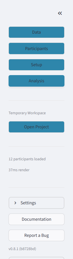
The sidebar bottom shows: Settings expander, Documentation button (links to rrational.readthedocs.io), Report a Bug button (links to GitHub Issues), and the version number with git commit hash (e.g., "v0.9.3 (a1b2c3d)").

---

Publication Checklist

Required for HRV Papers (Quigley 2024)

• Recording device and app used
• Recording duration per condition
• Artifact detection method (e.g., "Lipponen & Tarvainen 2019")
• Artifact correction method (e.g., "Kubios algorithm via NeuroKit2")
• Artifact rate per condition (mean ± SD)
• Number of excluded segments and exclusion criteria
• Beat count per condition
• Segment duration and overlap settings
• Which HRV metrics and why

---

Keyboard Shortcuts

Key	Action	Context
I	Toggle Signal Inspection mode / zoom	RR plot
R	Reset zoom	Signal Inspection mode
Left / Right	Pan the zoomed view	Signal Inspection zoom

---

Troubleshooting

Problem	Solution
"No data loaded"	Check files are in data/raw/ subfolder, verify ID pattern in Import Settings
"Section not detected"	Map events in Setup > Events, ensure start AND end events exist
"No validated sections found"	Go to Participants > Section Validation, click Save
Slow performance	Reduce plot resolution in Settings, close browser tabs

For installation issues, see Installation Guide.